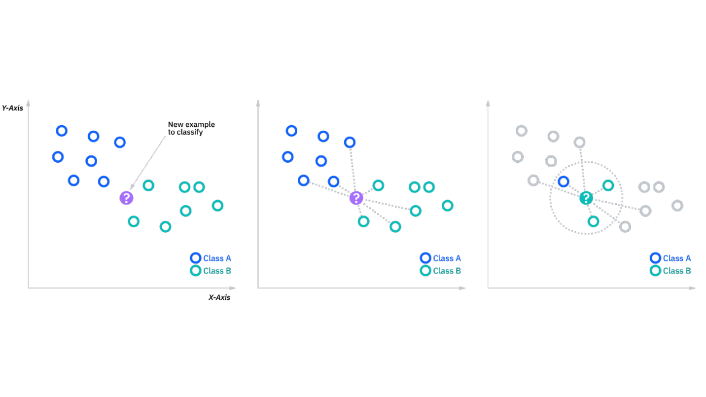
In the last two articles on K-Means Clustering and Hierarchical Clustering I focused on clustering algorithms (obviously!). But now, we move on to a different genre of algorithm with K-Nearest Neighbor or k-NN. k-NN is a classification algorithm that assumes that similar observations are near one another. This means, that given a new observation, the class label assigned to that point is the label that is most frequently present around that new observation. The ‘k’ in k-NN determines how many neighbors are we to look at before deciding on a class label. As can be seen in Figure A.1.1, we employ a 3-NN. Hence, for the new observation, we look at the three nearest neighbors. Since 2 out the 3 neighbors belong to Class B, we assign Class B to the new observation. Choosing the value of ‘k’ largely depends on the input data for e.g., data with huge number of outliers will be benefited from a higher value of ‘k’. However, larger values of ‘k’ can lead to high bias and low variance. Therefore, its a tradeoff that the user needs to be careful about.
 |
|---|
| Figure A.1.1 |
Data Analysis
Unlike the previous two algorithms - K-Means and Hierarchical Clustering which are unsupervised clustering algorithms, k-NN is a supervised classification algorithm. This means that -
- We are no longer clustering given observations; instead we are classifying a new observation based on a given set of observations.
- We now need a label corresponding to our observations.
Due to this, we now have to change the data we can use for the analysis for k-NN. We will start with our data variable from the K-Means article, which contains the pre-processed data. Let look at the data once again using head(data).
  Channel Fresh Milk Grocery Frozen Detergents_Paper Delicassen
1       2 12669 9656    7561    214             2674       1338
2       2  7057 9810    9568   1762             3293       1776
3       2  6353 8808    7684   2405             3516       7844
4       1 13265 1196    4221   6404              507       1788
5       2 22615 5410    7198   3915             1777       5185
6       2  9413 8259    5126    666             1795       1451
For k-NN, we will use this entire data. In this, our class label will be the “Channel” column and the rest of the six columns will be our predictor variables.
Now, we have to divide this dataset into Training and Testing.
# Split into training and testing dataset
n <- nrow(data)
reorder <- sample.int(n = n, size = n, replace = FALSE)

train_test_split <- 0.75
set <- ifelse(test = (reorder < train_test_split * n), yes = 1, no = 2)

data_train <- data[set == 1, ]
data_test <- data[set == 2, ]

# Get target variable in a separate dataframe
data_train_pred <- subset(data_train, select = -c(Channel))
data_train_tgt <- subset(data_train, select = c(Channel))
data_test_pred <- subset(data_test, select = -c(Channel))
data_test_tgt <- subset(data_test, select = c(Channel))
In the above code, we split the data using a 3:1 ratio. We have to create separate variables for predictor and target variables. We have 329 observations in our training data and 111 observations in our testing data. Now, just like the clustering algorithms, we need to scale our data. We can scale our training data like usual, but we need to scale our testing data using the mean and standard deviation that we used to scale our training data. This is due to the fact that, in real world, we dont know our test data. All we have is the training data, hence, when scaling a new observation, we can scale it using the parameters of our original set of observations.
# Scale the training data
s_data_train_pred <- scale(data_train_pred)

# Scale the test data using parameters from the training data
s_data_test_pred <- scale(data_test_pred,
                        center = attr(s_data_train_pred,
                                        "scaled:center"),
                        scale = attr(s_data_train_pred,
                                        "scaled:scale"))
k-NN in R
We will now implement k-NN in R using the knn() function, which is provided in the class library. knn() takes in four inputs - predictor variables for training data, predictor variables for test data, target variable for training data and the value for ‘k’. For now, we will follow the rule of thumb to use \(k = \sqrt{n}\) where n is the number of observations in the training data. This generally works and is good enough to give a baseline result for our data.
> # Looking for optimal value
> sqrt(nrow(data_train_pred))
[1] 18.13836
Given this, we can use \(k=18\).
knn_pred <- knn(train = s_data_train_pred,
                test = s_data_test_pred,
                cl = data_train_tgt[, 1],
                k = 18)
We can evaluate this by comparing the results to our test target variables
> # Evaluation
> matrix <- table(knn_pred, data_test_tgt[, 1])
> matrix

knn_pred  1  2
        1 63  4
        2  8 36
> (63+36)/111
[1] 0.8918919
The accuracy that we get from our model is 89.19%, which is quite good.
Analysis for ‘k’
In the previous section, we got an accuracy of 89.19% with \(k=18\). However, now we should run our previous code in a loop to see if there is a more optimal value of ‘k’ we can find. For this, we will just use our previous code and add it inside a for loop.
# Maximal value of 'k'
k_max <- 20

# Matrix to hold the values of accuracies
acc_record <- matrix(NA, nrow = k_max, ncol = 1)

# Looping for all values of k
for (r in 1:k_max) {
    # KNN
    knn_pred <- knn(train = s_data_train_pred,
                    test = s_data_test_pred,
                    cl = data_train_tgt[, 1],
                    k = r)

    # Evaluation
    matrix <- table(knn_pred, data_test_tgt[, 1])

    # accuracy = (TP + FN)/(Total number of points)
    acc <- (matrix[1] + matrix[4]) /
        (matrix[1] + matrix[2] + matrix[3] + matrix[4])

    # Store the current accuracy
    acc_record[r, 1] <- acc
}

# Plot Accuracy vs 'k'
plot(1:k_max, acc_record, type = "b",
    xlab = "Value of 'k'",
    ylab = "Accuracy")
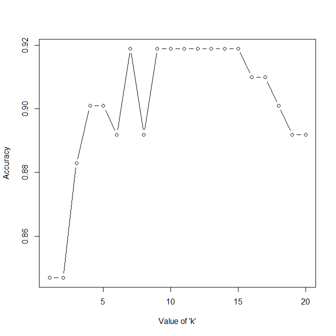
The result of the above plot can be seen in Figure A.1.2. From the plot we can observe that our rule of thumb ‘k’ gave a pretty good result. However, if we reduce it to \(k=15\), we can increase the accuracy to 91.89%. However, it is important to remember that currently we are using a very small amount of data to “train” our model. A more robust analysis would have been to use something like n-fold cross validation to get a more thorough idea about the optimal value of ‘k’.
 |
|---|
| Figure A.1.2 |
With this I complete the analysis on the Wholesale Dataset starting from two clustering algorithms and ending it with a classification technique.